library(tidyverse)
library(messy) # for creating messy data
library(naniar) # for assessing missing values
library(janitor) # Data cleaning
library(gt) #generating tables
library(gtExtras)
library(cowplot)Data Cleaning and Imputation
Handling Messy Data with tidyverse, janitor, naniar, and missForest
Project Summary
Goal: Demonstrate a systematic approach to data cleaning: fixing column names, standardizing inconsistent categorical values, handling missing data through Random Forest imputation, and validating results.
Data: The Iris dataset (150 observations, 3 species, 4 numeric features), deliberately messed up using the messy package to simulate real-world data quality issues.
Techniques: snake_case style standardization (janitor), string matching with case_when (dplyr), missingness assessment using (naniar), Random Forest imputation (missForest), and visualization with ggplot2.
Tools: R, tidyverse, janitor, naniar, missForest, cowplot, gt
Loading of libraries
The Iris dataset
The Iris dataset is one of the most famous datasets in statistics and machine learning. It was first introduced by the British biologist and statistician Ronald Fisher in 1936 in his paper “The use of multiple measurements in taxonomic problems.” The dataset consists of 150 samples of iris flowers from three different species: Setosa, Versicolor, and Virginica. Each sample includes four features/columns/variables: sepal length, sepal width, petal length, and petal width
Data cleaning & EDA
The explorations that I will conduct in this document will involve the following:
Messy column names
Improper variable types
Invalid or inconsistent values
Missing values
Non-standard data formats
Creating a Messy dataset
The messy package introduces realistic data quality problems: inconsistent column names, corrupted string values, changed data types, and missing values.
set.seed(123456)
messy_iris<-messy(iris)
messy_iris |>
  head() |>
gt()| Sepal.Length | Sepal.Width | Petal.Length | Petal.Width | Species |
|---|---|---|---|---|
| 5.1 | 3.5 | 1.4 | NA | setosa |
| 4.9 | 3 | NA | 0.2 | s$etosa |
| 4.7 | 3.2 | 1.3 | 0.2 | setosa |
| NA | 3.1 | 1.5 | 0.2 | NA |
| 5 | 3.6 | 1.4 | 0.2 | setosa |
| 5.4 | 3.9 | 1.7 | 0.4 | NA |
Key observations
- We can see that the column names are separated by “.” and are not in lower case. we are going to convert these to lower snake_case.
- Even before we search for missing values, we can note that the dataset has missing values
- Finally we can also see that the species column has more that three variations of the setosa (with over 68 different messed variations of the thre species).
- All columns are stored as character.
Understanding/Inspecting the Dataset
messy_iris |> #Checking the dimensions of the data (The data has 150 rows, and 5 columns)
  dim()
[1] 150 5messy_iris |> # Taking a quick look at our dataset
glimpse()Rows: 150
Columns: 5
$ Sepal.Length <chr> "5.1", "4.9", "4.7", NA, "5", "5.4 ", "4.6", "5", "4.4", …
$ Sepal.Width <chr> "3.5", "3", "3.2", "3.1 ", "3.6", "3.9", "3.4", "3.4", "2…
$ Petal.Length <chr> "1.4", NA, "1.3", "1.5 ", "1.4", "1.7", "1.4", "1.5", "1.…
$ Petal.Width <chr> NA, "0.2", "0.2", "0.2", "0.2 ", "0.4", "0.3", "0.2", NA,…
$ Species <chr> "setosa", "s$etosa", "setosa", NA, "setosa", NA, "setosa"…It can be immediately observed that all columns are of character type, and the species column needs standardisation.
messy_iris |>  # Understanding the column names of the dataset
  colnames()
[1] "Sepal.Length" "Sepal.Width" "Petal.Length" "Petal.Width" "Species" messy_iris |> # Checking for unique values of Species.
select(Species) |>
distinct() Species
1 setosa
2 s$etosa
3 <NA>
4 set)osa
5 s+et&osa
6 SETOSA
7 se+tosa
8 set_osa
9 s@etosa
10 s)eto!sa
11 $setosa
12 setos%a
13 set-osa
14 *setosa
15 s^e*tosa
16 s)etosa
17 (setosa
18 setos.a
19 se(tosa
20 setosa
21 se#t#o)sa
22 s-etosa
23 s_etosa
24 s&etosa
25 s^etosa
26 seto^sa
27 ^set.o(s-a
28 ver!sicolor
29 ver)sicolor
30 vers$icolor
31 ve%rsicol!or
32 ver$sicolor
33 versic(olor
34 versi(color
35 versi-color
36 versicolor
37 versicol(or
38 *versicolor
39 versic+olor
40 versi_co%lor
41 VERS!ICOLOR
42 versi$c$olor
43 versi%c%olor
44 versico&lor
45 ve^rsicolor
46 ^versicolor
47 ve.rsicolor
48 ver#sico!lor
49 $v%ersicolo_r
50 versicol#or
51 ve@rs(icolor
52 versicolor
53 ve@rsicolo%r
54 vers&icolor
55 v_e)rsicolo)r
56 ve(rsi.col*or
57 versico)lor
58 %versicolo#r
59 versi&col#o!r
60 versic^olor
61 *versico!lo.r
62 &vers)icolor
63 ver^sicolor
64 ver#sicolor
65 ve_rs#ic-olo$r
66 vers.icolor
67 virginica
68 @virginica
69 virginic@a
70 v-i*rg%i#nica
71 virgin*ica
72 virgi*nica
73 virgin&ica
74 v%irgini%ca
75 virgini+ca
76 virgini)ca
77 v.irginica
78 virgi(nic-a
79 -virginica
80 virg*inica
81 virginic$a
82 vir&gini(ca
83 v-irginica
84 virgi@nica
85 &virginica
86 virginica
87 vir@ginic)a
88 #virgin(ica
89 virg(inica
90 virg_i%nic^a
91 virginic.aThe dataset is supposed to have three different species of the flower namely; setosa, viginica, and versicolor. However, we can quickly note from code output that we have over 68 different variations of these species. Again, we are going to fix this too!!
Data Cleaning process
Step 1: Fix Column Names
clean_iris<-messy_iris |>
  clean_names()
clean_iris |>
  head(10)
sepal_length sepal_width petal_length petal_width species
1 5.1 3.5 1.4 <NA> setosa
2 4.9 3 <NA> 0.2 s$etosa
3 4.7 3.2 1.3 0.2 setosa
4 <NA> 3.1 1.5 0.2 <NA>
5 5 3.6 1.4 0.2 setosa
6 5.4 3.9 1.7 0.4 <NA>
7 4.6 3.4 1.4 0.3 setosa
8 5 3.4 1.5 0.2 setosa
9 4.4 2.9 1.4 <NA> setosa
10 4.9 3.1 <NA> 0.1 set)osaNote that our column names are now in lower case using the snake_case format. The next thing that we are going to do is ensure that the species column only has the three different values.
Step 2 : Standardise Species Values
head(clean_iris$species)[1] "setosa" "s$etosa" "setosa" NA "setosa" NA bad_setosa <- c( "setos)a", "setosa ", "setosa","setosa", "setosa", "setosa ", "seto_sa", "s&etosa", "setosa", "SETOSA", "setosa", "se(tosa", "setosa","setosa", "setosa","setosa","*setosa","set_osa","setosa", "se@tosa","setosa", "(s_etos.a", "set(osa","setos$a","seto-s(a","(SETOSA","setosa ", "s-eto%sa", "setosa","SETOSA", "seto.sa","setosa","setos^a", "setosa","set$osa", "setosa", "se+tosa","seto*sa", "S)ETOSA","setos*a", "setosa","set!osa","setosa","setosa","s@et#osa ","setosa","setosa")bad_versicolor<-c("versic(olor","ver@sicolor","versico_lor","ve#rsicolor","versicolor", "versico@lor","versicolor","versicolor","versicolor","versicolor","versicolor","vers_i%c#ol%or", "V*ERSICOLOR","ver!sicolor","+versicolo^r","versicolor","versico)l^or","versicol^or","ve&rsicolor","versicolor","$vers+icolor","versicolor ",")versicolor", "versicolor","versicolor","versicolor","versicolor ","ver&sicolor ","versico(lo$r","versi_color","versicolor","vers-ic.ol%o&r", "versicolor","versicolor", "versicolor","*versicolor","versicolor","versicol!or","&versicolor","%versicol%or ", "v%ersicolor","v+ersicolor")bad_virginica <- c("virginica","vir!ginica","virginica","VIRGINICA","virginica","virginica",
"virginica","virg^inica","virginica","$virg(inica","virginica","virginica ","virginica", "virginica","virgini+ca","vir-ginica", "virginica","virginica","virgin!ica","virginica", ".virginic#a","virginica","virginic_a","virginica","v(irgi$nica","virginica","virginic#a", "vir.gini@ca","virginica ","v#irgini(ca", "virginica","virginica","virginica","virginica", "virgi^nica","virginica","virginica","virginica","VIRGINICA","virginica","virginica")The code below, is going to replace bad species with the right value using dplyr case_when function
clean_iris<-clean_iris |>
   mutate(species_clean = case_when(species %in% bad_setosa ~ "setosa",
                                    species %in% bad_versicolor ~ "versicolor",
                                    species %in% bad_virginica ~ "virginica"))

unique(clean_iris$species_clean)
[1] "setosa" NA "versicolor" "virginica" Species column now only contains the three designated species
Step 3 : Converting Data Types
clean_iris<-clean_iris |>
  mutate(across(c(sepal_length,
                  sepal_width,
                  petal_length,
                  petal_width),as.numeric),
         species_clean=factor(species_clean))

clean_iris |>
  glimpse()
Rows: 150
Columns: 6
$ sepal_length <dbl> 5.1, 4.9, 4.7, NA, 5.0, 5.4, 4.6, 5.0, 4.4, 4.9, 5.4, 4.…
$ sepal_width <dbl> 3.5, 3.0, 3.2, 3.1, 3.6, 3.9, 3.4, 3.4, 2.9, 3.1, 3.7, 3…
$ petal_length <dbl> 1.4, NA, 1.3, 1.5, 1.4, 1.7, 1.4, 1.5, 1.4, NA, 1.5, 1.6…
$ petal_width <dbl> NA, 0.2, 0.2, 0.2, 0.2, 0.4, 0.3, 0.2, NA, 0.1, 0.2, 0.2…
$ species <chr> "setosa", "s$etosa", "setosa", NA, "setosa", NA, "setosa…
$ species_clean <fct> setosa, NA, setosa, NA, setosa, NA, setosa, setosa, seto…After conversion, we now have numeric columns converted to double precision, Species (character) converted to factor.
Checking for missingness in Iris dataset
clean_iris |>
  miss_var_summary() |>
gt()| variable | n_miss | pct_miss |
|---|---|---|
| species_clean | 87 | 58 |
| petal_length | 22 | 14.7 |
| petal_width | 20 | 13.3 |
| sepal_length | 19 | 12.7 |
| species | 12 | 8 |
| sepal_width | 11 | 7.33 |
vis_miss(clean_iris)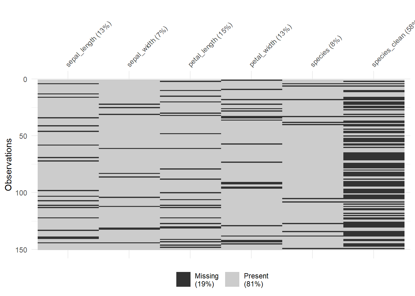
We have over 57.3% of missing dataset for species. There are many ways of handling missing values including list-wise deletion to drop all missing values. This is not the recommended method.
Imputation with missForest
There are many ways of working with missing values including methods such as listwise deletion, pairwise deletion, imputation etc. In this section we are going to use imputation by employing a package; missForest, which uses random forest to train data of observed values of data matrix to predict missing values.
#install.packages("missForest")
library(missForest)

iris_impute<-clean_iris |>
  select(-species) |>
  mutate(across(c(sepal_length,
                  sepal_width,
                  petal_length,
                  petal_width), as.numeric),
         species_clean = as.factor(species_clean))


iris_imputed<-missForest(iris_impute,xtrue = ,maxiter = 10,ntree = 100,verbose = FALSE)

df_imputed<-iris_imputed$ximp

df_imputed |>
  miss_var_summary() |>
gt() | variable | n_miss | pct_miss |
|---|---|---|
| sepal_length | 0 | 0 |
| sepal_width | 0 | 0 |
| petal_length | 0 | 0 |
| petal_width | 0 | 0 |
| species_clean | 0 | 0 |
Even though imputing datasets (multiple imputation) is better than methods like list wise deletion, along with it comes ethical implications especially for identity data.
iris_imputed$OOBerror NRMSE PFC
0.13960904 0.01587302 Out of the bag error rates for both the categorical and numerical predictions indicating reliable imputation.
Validation: Comparing Imputed vs Original Data
In this section we will compare distributions of the imputed dataset against the original Iris dataset to check whether or not imputation preserved the original data structure.
plot_sl_1<-df_imputed |>
  ggplot(aes(x = sepal_length)) +
  geom_histogram()+
  theme_bw() +
  labs(title = "Histogram - Imputed data")
iris_sp1<-iris |>
  ggplot(aes(x = Sepal.Length))+
  geom_histogram()+
  theme_bw()+
  labs(title = "Histogram - original data")

plot_sl_2<-df_imputed |>
  ggplot(aes(sample = sepal_length))+
  stat_qq()+
  stat_qq_line(color = "red")+
  theme_bw() +
  labs(title = "Q-Q plot for imputed data")

iris_sl_2<-iris |>
  ggplot(aes(sample = Sepal.Length))+
  stat_qq()+
  stat_qq_line(color = "red")+
  theme_bw() +
  labs(title = "Q-Q Plot original data")

cowplot::plot_grid(plot_sl_1, iris_sp1,plot_sl_2,iris_sl_2, ncol = 2)
`stat_bin()` using `bins = 30`. Pick better value `binwidth`.
`stat_bin()` using `bins = 30`. Pick better value `binwidth`.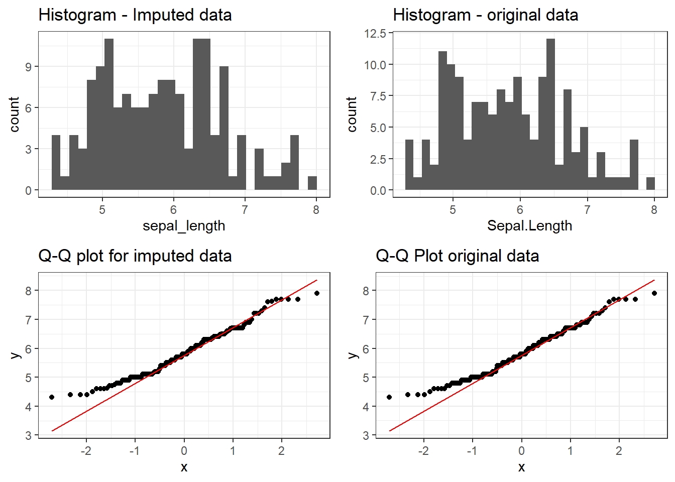
The imputed distributions closely match that of the original dataset, confirming that missForest preserved the underlaying data structure.
VISUALISATION
df_imputed |>
  ggplot(aes(x = sepal_length,y = petal_width))+
  geom_point(aes(colour = species_clean, size = petal_length), alpha = 0.5) +
  scale_color_manual(values = c("#00AFBB", "#e7b800","#FC4E07"))+
  scale_size(range = c(0.5, 12)) +
  theme_bw()+
  labs(title = "Plot showing Petal width against Petal length")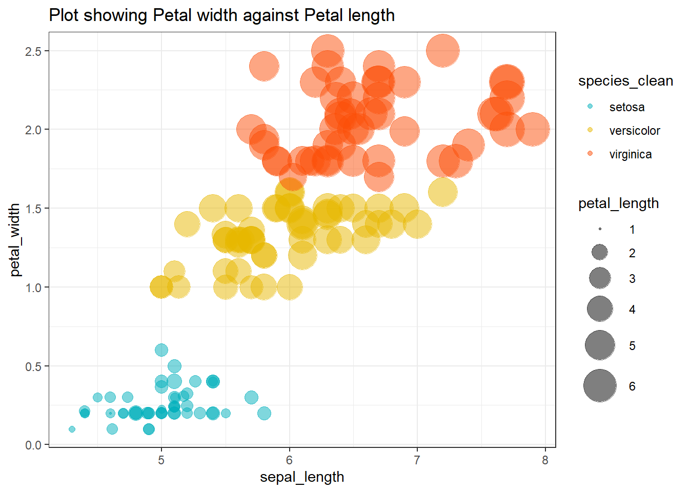
The scatter plot shows clear clustering by species, with Setoisa separating distinctly from both Versicolor and Virginica. This confirms that the imputed dataset retains the original grouping or classification structure.