MLearning

Project Summary

Goal: Predict diabetes status from demographic and clinical risk factors using the NHANES dataset.

Data: National Health and Nutrition Examination Survey collected in the US. Variables include age, BMI, direct cholesterol, marital status, and gender.

Models: Logistic Regression and Random Forest (tidymodels framework).

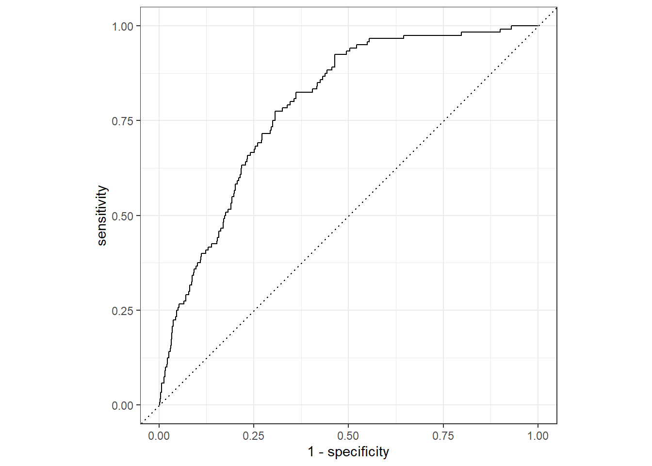
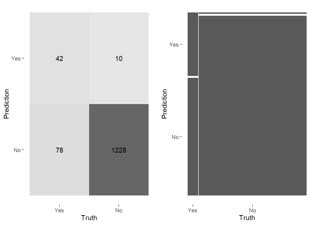
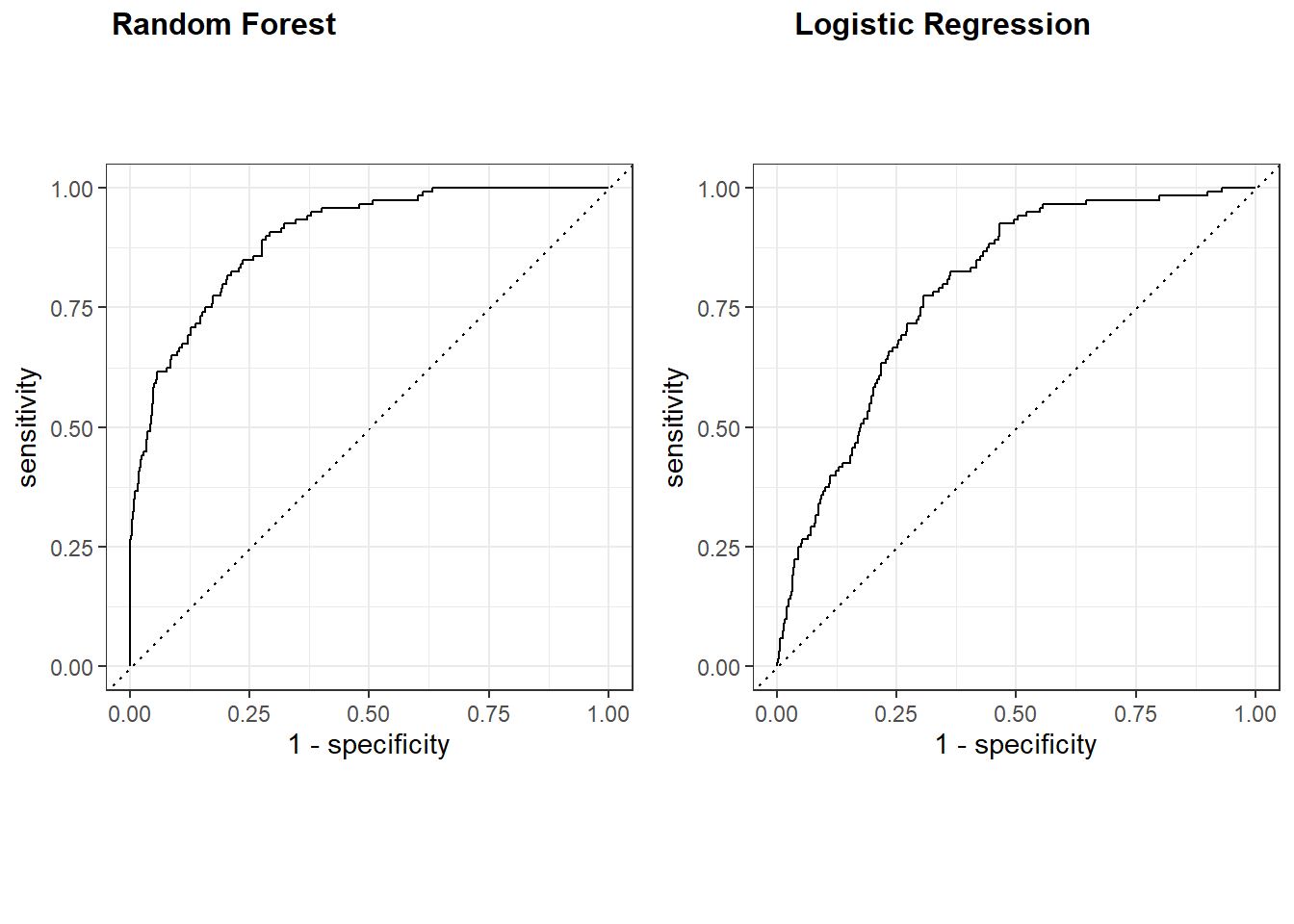
Key Finding: Random Forest outperformed logistic regression across all metrics. Sensitivity improved from 4% (logistic regression) to 34% (Random Forest), with ROC-AUC of 0.89. Both models struggled with the minority class due to class imbalance.

Tools: R, tidymodels, ranger, ggstatsplot, cowplot, gtsummary

Introduction

In this project we will use the NHANES dataset to predict diabetes given the available risk factors. The National Health ans Nutrition Survey is a a program in the US designed to assess the health and nutritional status pf adults, and children in the US. The data includes demographic, socio-economic, dietary, and health-related information.

Loading packages including the dataset.

Data Preparation

We are going to save the dataset into the nhanes_df object to maintain the original dataset intact.

nhanes_df<-NHANES |> 
  select(Diabetes,DirectChol,BMI,MaritalStatus,Age,Gender) |>
  drop_na() |> # Assuming variables are missing completely at Random
  clean_names()

# Changing the levels for appropriate analysis
nhanes_df<-nhanes_df |> 
  mutate(diabetes=factor(diabetes, 
                         levels = c("Yes", "No"))) |> 
           glimpse()

Rows: 6,786
Columns: 6
$ diabetes       <fct> No, No, No, No, No, No, No, No, No, No, No, No, No, No,…
$ direct_chol    <dbl> 1.29, 1.29, 1.29, 1.16, 2.12, 2.12, 2.12, 0.67, 0.96, 1…
$ bmi            <dbl> 32.22, 32.22, 32.22, 30.57, 27.24, 27.24, 27.24, 23.67,…
$ marital_status <fct> Married, Married, Married, LivePartner, Married, Marrie…
$ age            <int> 34, 34, 34, 49, 45, 45, 45, 66, 58, 54, 58, 50, 33, 60,…
$ gender         <fct> male, male, male, female, female, female, female, male,…

Train/Test Split

In the code below, we are splitting our data into training and testing sets (0.8, 0.2) and stratify by the diabetes to preserve class proportions.

set.seed(123) #For reproducubility
ml_split<-initial_split(nhanes_df,
                        prop = 0.8,
                        strata = diabetes)

ml_training<-ml_split |> 
  training()

ml_test<-ml_split |>
  testing()

Logistic Regression

lr_model<-logistic_reg() |> 
  set_engine("glm") |> 
  set_mode("classification") 

Correlation Check

ml_training |> 
  select_if(is.numeric) |> 
  ggcorrmat(colors = c("#B2182B", "White", "#4D4D4D"),
            title = "Colleration Matrix"
            )

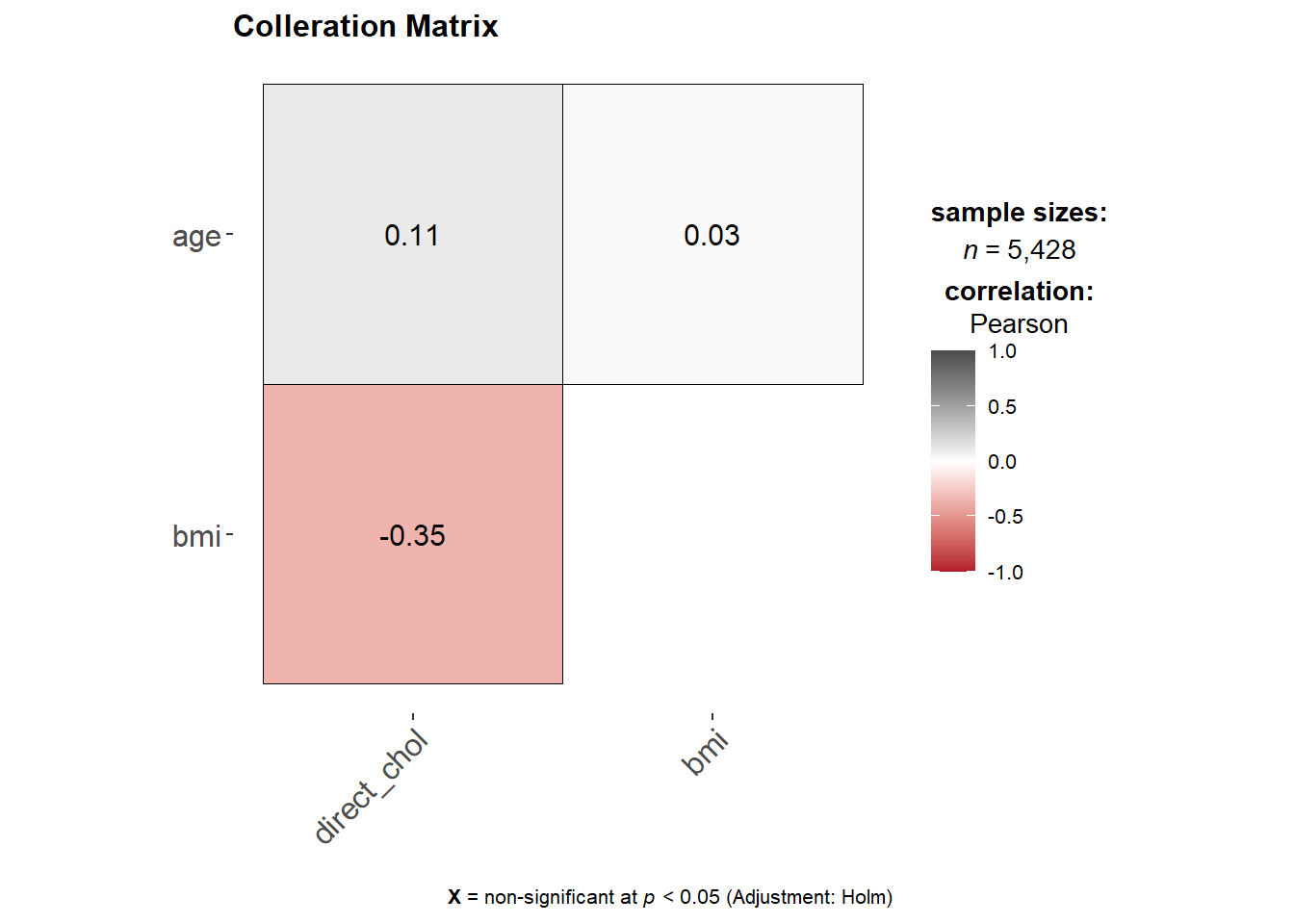
Using the hypothetical threshold of 0.8, we can conclude that the predictors are not collerated. In the code below, we are going to fit both models using the fit function. After which we are going to collect and combine predictions, and load them.

In the code below we are going to specify a recipe object after which we will add steps for engineering our features (feature engineering). The steps are to preprocess the data into a form that will allegedly improve our analysis.

Workflow and Fit

set.seed(123)
lr_recipe<-recipe(diabetes~.,data = ml_training) |>
  step_log(all_numeric()) |> 
  step_normalize(all_numeric()) |> #Centering and scaling
  step_dummy(all_nominal(), -all_outcomes())

lr_worflow<-workflow() |> 
  add_model(lr_model) |> 
  add_recipe(lr_recipe)

set.seed(123)
lr_worflow_fit<-lr_worflow |> 
  last_fit(split = ml_split)

lr_worflow_fit |> 
  collect_metrics()

# A tibble: 3 × 4
  .metric     .estimator .estimate .config             
  <chr>       <chr>          <dbl> <chr>               
1 accuracy    binary        0.909  Preprocessor1_Model1
2 roc_auc     binary        0.790  Preprocessor1_Model1
3 brier_class binary        0.0743 Preprocessor1_Model1

lr_resultss<-lr_worflow_fit |> 
  collect_predictions()

lr_resultss

# A tibble: 1,358 × 7
   .pred_class .pred_Yes .pred_No id                .row diabetes .config       
   <fct>           <dbl>    <dbl> <chr>            <int> <fct>    <chr>         
 1 No             0.0774    0.923 train/test split     4 No       Preprocessor1…
 2 No             0.0941    0.906 train/test split    10 No       Preprocessor1…
 3 No             0.103     0.897 train/test split    11 No       Preprocessor1…
 4 No             0.101     0.899 train/test split    12 No       Preprocessor1…
 5 No             0.112     0.888 train/test split    14 No       Preprocessor1…
 6 No             0.0235    0.976 train/test split    15 No       Preprocessor1…
 7 No             0.207     0.793 train/test split    19 No       Preprocessor1…
 8 No             0.131     0.869 train/test split    22 Yes      Preprocessor1…
 9 No             0.122     0.878 train/test split    24 Yes      Preprocessor1…
10 No             0.0877    0.912 train/test split    28 No       Preprocessor1…
# ℹ 1,348 more rows

Logistic Regression Results

Confusion Matrix

In this section we are going to visualize the model results. We will start with the confusion matrix.

set.seed(123)
lr_resultss |> 
  conf_mat(truth = diabetes,
           estimate = .pred_class)

          Truth
Prediction  Yes   No
       Yes    4    8
       No   116 1230

• The logistic regression correctly classifies 1,237 out of 1,358 individuals (91%). 116 false negatives and 8 false positives.

  Performance Metrics

set.seed(112)
lr_metric<-metric_set(sens,accuracy, yardstick::spec)



lr_resultss |> 
  lr_metric(truth = diabetes, 
            estimate = .pred_class)

# A tibble: 3 × 3
  .metric  .estimator .estimate
  <chr>    <chr>          <dbl>
1 sens     binary        0.0333
2 accuracy binary        0.909 
3 spec     binary        0.994 

set.seed(123)
lr_resultss |>
  roc_curve(truth = diabetes,.pred_Yes) |>
  autoplot()

roc_auc(lr_resultss, truth = diabetes, .pred_Yes)

# A tibble: 1 × 3
  .metric .estimator .estimate
  <chr>   <chr>          <dbl>
1 roc_auc binary         0.790

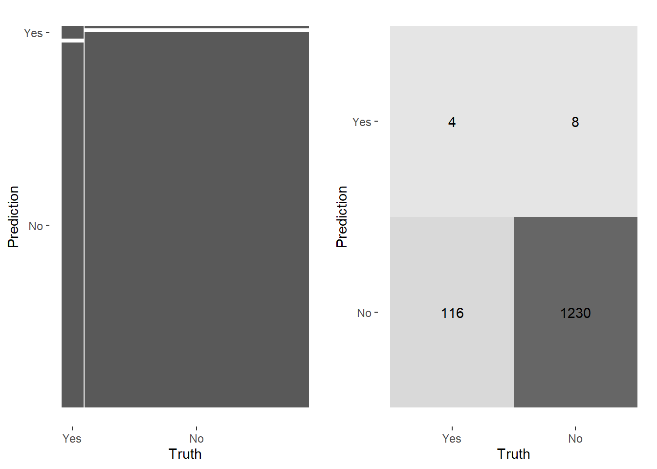
set.seed(123)
heatmap_lr<-conf_mat(lr_resultss, truth = diabetes, estimate = .pred_class) |> 
  autoplot(type = "heatmap")


mosaic_lr<-conf_mat(lr_resultss, truth = diabetes, estimate = .pred_class) |> 
  autoplot(type = "mosaic")

cowplot::plot_grid(mosaic_lr,heatmap_lr)

The 91.1% accuracy is misleading. The model predicts negative cases well (high specificity) but identifies only 4 out of 120 positive cases. Accuracy alone is not a useful metric here due to class imbalance.

set.seed(123)
roc_auc(lr_resultss,truth = diabetes,.pred_Yes)

# A tibble: 1 × 3
  .metric .estimator .estimate
  <chr>   <chr>          <dbl>
1 roc_auc binary         0.790

lr_roc_plot<-lr_resultss |> 
  roc_curve(truth = diabetes, .pred_Yes) |> 
  autoplot()
  
lr_roc_plot

Random Forest

Logistic regression failed to correctly identify positive cases. Random Forest offers more flexibility for nonlinear relationships and imbalanced data.

Model Specification

rf<-rand_forest() |> 
  set_args(mtry = 9) |> 
  set_engine("ranger", importance = "impurity") |> 
  set_mode("classification")

set.seed(123)
rf_recipe<-recipe(diabetes~.,data = ml_training) |> 
  step_log(all_numeric()) |> 
  step_normalize(all_numeric()) |> 
  step_dummy(all_nominal(),-all_outcomes())

rf_workflow<-workflow() |> 
  add_model(rf) |> 
  add_recipe(rf_recipe)

set.seed(123)
rf_wrkflw_fit<-rf_workflow |> 
  tune::last_fit(split = ml_split)

rf_wrkflw_fit |> 
  collect_metrics()

# A tibble: 3 × 4
  .metric     .estimator .estimate .config             
  <chr>       <chr>          <dbl> <chr>               
1 accuracy    binary        0.935  Preprocessor1_Model1
2 roc_auc     binary        0.896  Preprocessor1_Model1
3 brier_class binary        0.0551 Preprocessor1_Model1

rf_results<-rf_wrkflw_fit |> 
  collect_predictions()

Random Forest Results

set.seed(123)
mosaic_rf<-rf_results |> 
  conf_mat(truth = diabetes,.pred_class) |> 
  autoplot(type = "mosaic")

heatmap_rf<-rf_results |> 
  conf_mat(truth = diabetes,.pred_class) |>
  autoplot(type = "heatmap")
  
cowplot::plot_grid(heatmap_rf,mosaic_rf)

set.seed(123)
rf_metrics<-metric_set(yardstick::sens, yardstick::spec, yardstick::accuracy)


lr_resultss |> 
  rf_metrics(truth = diabetes, 
            estimate = .pred_class)

# A tibble: 3 × 3
  .metric  .estimator .estimate
  <chr>    <chr>          <dbl>
1 sens     binary        0.0333
2 spec     binary        0.994 
3 accuracy binary        0.909 

rf_results |> 
  rf_metrics(truth = diabetes, estimate = .pred_class)

# A tibble: 3 × 3
  .metric  .estimator .estimate
  <chr>    <chr>          <dbl>
1 sens     binary         0.35 
2 spec     binary         0.992
3 accuracy binary         0.935

rf_results |> 
  roc_auc(truth = diabetes,.pred_Yes)

# A tibble: 1 × 3
  .metric .estimator .estimate
  <chr>   <chr>          <dbl>
1 roc_auc binary         0.896

rf_roc_plot<-rf_results |> 
  roc_curve(truth = diabetes,.pred_Yes) |> 
  autoplot()

Model comparison

cowplot::plot_grid(rf_roc_plot, lr_roc_plot,labels = c("Random Forest", "Logistic Regression"),label_size = 12)

Random Forest outperforms logistic regression on all metrics:

The Random Forest improves sensitivity from 4% to 34%. The model still misses 64% of positive cases due to class imbalance.

Metric	Logistic Regression	Random Forest
Accuracy	0.91	0.93
Sensitivity	0.04	0.35
Specificity	0.99	0.99
ROC-AUC	0.83	0.89

Prediction Example (Use case)

patient1<-tribble(~age,~bmi,~direct_chol,~marital_status,~gender,
                  40,27.3,1.5,"Divorced","female")

rf_pred<-rf_wrkflw_fit |> 
  extract_workflow()

predict(rf_pred, new_data = patient1)

# A tibble: 1 × 1
  .pred_class
  <fct>      
1 No         

The model predicts this patient does not have diabetes. Given the model’s high specificity, negative predictions are reliable.

Limitations and Next Steps

This analysis skipped hyperparameter tuning (k-fold cross validation) and did not address class imbalance through oversampling (SMOTE) or threshold adjustment. These are the clear next steps for improving sensitivity on the minority class.